Tutorial MetaTOR
In this notebook we will give an example on how to run MetaTOR [1] in order to bin metganomics assembly into MAGs and explain the output of the pipeline.
Table of contents
Input data
In this analysis, we will use the metaHiC sample from Marbouty et al., eLife, 2021. The accession number of the fastq sequences is SRR13435231 and the assembly accession number is ASM1314648v1 in the BioProject PRJNA627086 on the NCBI database:
Forward metaHiC reads: hic_reads_for.fastq.gz
Reverse metaHiC reads: hic_reads_rev.fastq.gz
Assembly sequences: assembly.fa
Here the assembly has been made using proximity ligation library (PE Illumina sequencing: 2x75bp, NextSeq500). Before building the assembly reads were filtered and trimmed using Cutadapt (v1.9.1). Here the assembly have been build using Megahit (v1.1.1.2) with default paramters.
However, it’s better to use a short reads (PE reads shotgun) library to build a better assembly. For example, you can use Megahit (v1.2.9) or Spades (v3.15.2) as below to build your own assembly of your sample.
Using Megahit [2]:
megahit -1 shotgun_reads_for.fastq.gz -2 shotgun_reads_rev.fastq.gz -o assembly.fa --min-contig-len 500
Using Spades [3] (more advanced tutorial is available here):
metaspades.py 1 shotgun_reads_for.fastq.gz -2 shotgun_reads_rev.fastq.gz -o assembly_folder
For Spades assembly we advise to set a minimum contig length threshold of 500bp as MetaTOR won’t be able to bin efficiently smaller contigs.
A. Quick start
1. Simplest command
The simplest way to run metaTOR consist to run the full pipeline in one command with the default parameters:
metator pipeline -1 hic_reads_for.fastq.gz -2 hic_reads_rev.fastq.gz -a assembly.fa -o metator_folder --threads 16
INFO :: Minimum mapping quality: 30
INFO :: Enzyme: None
INFO :: Normalization: empirical_hit
INFO :: Partition algorithm: louvain
INFO :: Partition iterations: 100
INFO :: Overlapping parameter: 0.8
INFO :: Recursive partition iterations: 10
INFO :: Recursive overlapping parameter: 0.9
INFO :: Build index from the given fasta.
INFO :: Alignment of hic_for.fastq.gz:
[bam_sort_core] merging from 0 files and 16 in-memory blocks...
INFO :: Alignment of hic_rev.fastq.gz:
[bam_sort_core] merging from 0 files and 16 in-memory blocks...
INFO :: 44694905 forward reads aligned and 43649065 reverse reads aligned
INFO :: Merging the pairs:
INFO :: 38922357 pairs aligned.
INFO :: Information of alignment_0.pairs:
INFO :: 38922357 contacts in the library.
INFO :: 15243120 contacts inter-contigs in the library.
INFO :: 3D ratio : 0.39162890366582886

INFO :: Start iterations:
INFO :: Iteration in progress: 0
[...]
INFO :: Iteration in progress: 99
0.909622

INFO :: Detect core bins:
INFO :: 3467 core bins were found.
INFO :: Detect overlapping bins:
INFO :: 2131 overlapping bins were found.
INFO :: Extract bins:
INFO :: 61 bins have been extracted
INFO :: Total size of the extracted bins: 294.519Mb
INFO :: Start CheckM validation.
[...]
INFO :: 106 bins have been kept after the recursive iterations.
INFO :: Total size of the extracted bins: 270076511
INFO :: HQ MAGs: 37 Total Size: 97198990
INFO :: MQ MAGs: 32 Total Size: 84773041
INFO :: LQ MAGs: 9 Total Size: 17679996
INFO :: Contaminated potential MAGs: 11 Total Size: 47487326
INFO :: Others bins: 17 Total Size: 22937158
2. Main output files
The Software will give you the output in the metator folder, the full description of the output are available in the README. The main output file is the final_bin directory with one fasta for each final bin. Moreover, in the bin summary file, see example below, you will find all informations known by the algorithm on the MAGs.
| lineage | completness | contamination | size | contigs | N50 | longest_contig | GC | coding_density | taxonomy | HiC_Coverage | |
|---|---|---|---|---|---|---|---|---|---|---|---|
| MetaTOR_1_3 | f__Lachnospiraceae | 99.52 | 5.57 | 4119470 | 469 | 40705 | 112608 | 46.37 | 88.85 | k__Bacteria;p__Firmicutes;c__Clostridia;o__Clostridiales;f__Lachnospiraceae | 2.14E+02 |
| MetaTOR_1_4 | o__Clostridiales | 98.66 | 0.57 | 2859491 | 131 | 66245 | 143889 | 37.22 | 89.63 | k__Bacteria;p__Firmicutes;c__Clostridia;o__Clostridiales;f__Lachnospiraceae_2;g__Lachnospira | 6.04E+01 |
| MetaTOR_2_0 | o__Clostridiales | 92.95 | 10.37 | 3471666 | 1456 | 4479 | 85988 | 47.64 | 88.54 | k__Bacteria;p__Firmicutes;c__Clostridia;o__Clostridiales;f__Lachnospiraceae;g__Blautia | 3.59E+01 |
If give you some binning plot summary too:
| Bins completion/contamination distribution | Bins size quality distribution |
|---|---|
 |
 |
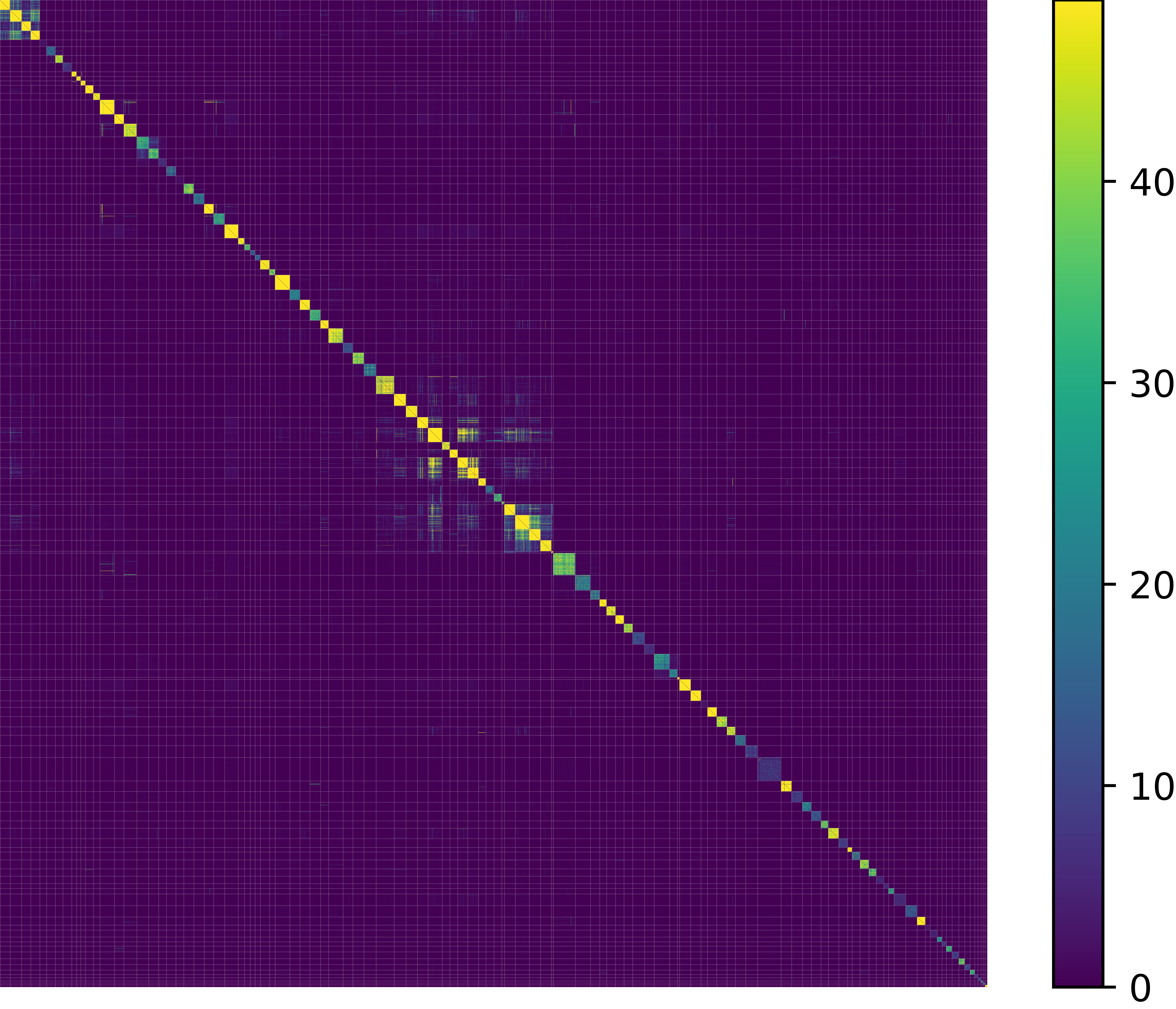
Another plot is the heatmap of the final bin network. It display the integrity inside a MAG and the noise between MAGs. All the bins of more than 500kb are represented. The order of the bins is the same as in the bin_summary.txt file. The binning size is 50kb.
 network_heatmap
B. A multiple modules pipeline
This command will take some time as the Software will run all the steps with this. For the 140,409 contigs assembly example (314Mb) with 56 millions reads with 16 threads, it will take around 74.2 minutes and up to around 40G memory usage (CheckM validation step). However it’s possible to skip some step if you don’t need them or you have already done them to speed up the process.
1. Choose your starting point
 metator_pipeline_figures
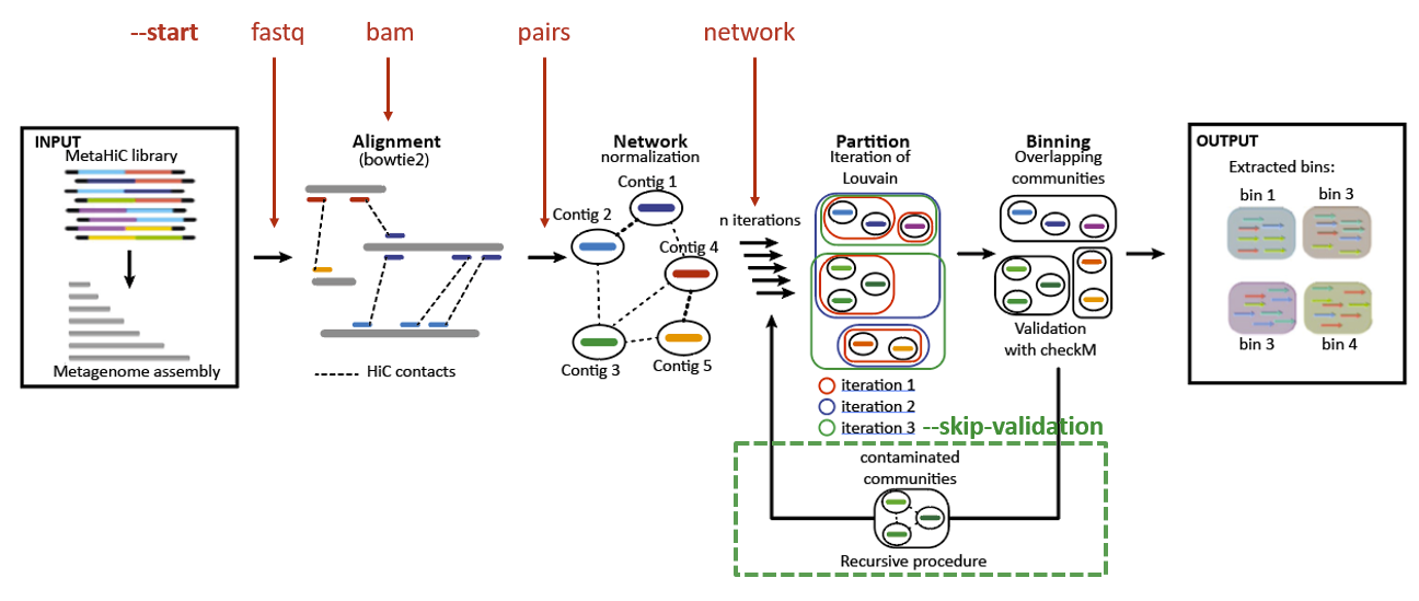
One of the longest step is the alignemnent of the reads and the computation of the pairs file. Moreover, currently metaTOR use only bowtie2 to do the alignment with the –very-sensitive-local parameters to align the reads. You may already have a bam or a pairs file from another anlysis, or just want to use another aligner software, or different parameters of bowtie2. That’s why it’s possible to start at different stage with the --start parameter. There are four possible start:
fastq: The default one with HiC forward and reverse reads fastq files (with this start it’s possible to give the fasta or the bowtie2 index).
metator pipeline -1 hic_reads_for.fastq.gz -2 hic_reads_rev.fastq.gz -a assembly_bowtie2_index -S fastq
bam: To avoid the alignment. Currently the only accecpted input is to seperate bam with the forward and reverse aligned separately. It could allow you to use different aligner or aligner parameters. WARNING: bam files need to be sorted on the reads ids in both files.
metator pipeline -1 for.bam -2 rev.bam -a assembly.fa -S bam
pair: One pair file which follow the official specification of the pairix format. This step allowed you to align simultaneously align both forward and reverse reads. However, you have to be careful as HiC pairs could be paires as unconcordant reads as they could be chimeric.
metator pipeline -1 alignment.pairs -a assembly.fa-S pairs
network: A three column tsv network file with the first contig ID (1-based ids) the second contig ID and the normalised contact. This step allow you to use another custom normalization.
metator pipeline -n network.txt -a assembly.fa -S network
2. Skip the validation module
The recursif binning of metaTOR used checkM to check the contamination of the MAGs and apply a recursif clustering of the contigs in the contaminated MAGs. This step is a key step to clean the obtained MAG automatically. However, checkM needs a 40G memory usage. If you do not want to launch it you could skip the validation process and so the recursive binning of metaTOR:
metator pipeline -1 hic_reads_for.fastq.gz -2 hic_reads_rev.fastq.gz -a assembly_bowtie2_index -v
3. Launch the modules separately
It’s also to launch the modules separately sequentially (the network module have the three first start stage option):
metator network -1 for.bam -2 rev.bam -a assembly.fa
metator partition -c contig_data_network.txt -n network.txt -a assembly.fa
metator validation -c contig_data_partition.txt -n network.txt -a assembly.fa -f overlapping_bin
C. Advanced parameters
1. Digestion site
The reads came from a metaHiC experiment where different restriction enzyme could have been used. MetaTOR is able to integrate in the contig data information the number of restriction sites of each contigs.
Normalization: As HiC coverage depends on the density of restriction site, this data could be useful for normalization method using model based on the coverage of the contigs. The default normalization does not need it as we do not train any model and just use the geometric mean of the intra-contig contacts to normalize the inter-contig contacts. Indeed, we expect the number of intra-contig contacts to depends on the size, the restriction site density and the abundance of contig as the inter-contigs contacts.
Ligation sites: The restriction enzyme could also be used to preprocess the reads. Indeed, HiC reads could be chimeric, i.e. an ligation event could occur inside one read. If a ligation event occur in the reads, the aligner will only map the biggest half of the read and assign a bad mapping quality on the read. To avoid to loose these reads it’s possible to use an iterative alignment (start with only 20 first bases of the reads and add iteratively 20bp until the read is mapped, or maximum length is reached). Another possibility is to first preprocess the reads by cutting them on the ligation sites. For example, for HpaII, the restriction site is CCG and the ligation site will CCGCGG. Furthermore,CCGCGG if a ligation event is detected it’s possible to create two pairs from the previous one with each part of the cutting read. This preprocess is especially useful with “long” PE sequencing (2x100bp or longer) and if the restriction sites density is high (1 every 100bp). A module to preprocess the data is available in hicstuff [4]:
hicstuff digest -1 hic_reads_for.fastq.gz -2 hic_reads_for.fastq.gz -p hic_reads_cutsite -e HpaII
The module returns two new digested fastq with prefix given (here hic_reads_cutsite), which could be use as input data. In this example the preprocess haven’t been done as the HiC reads are only 2x35bp.
2. Binning parameters
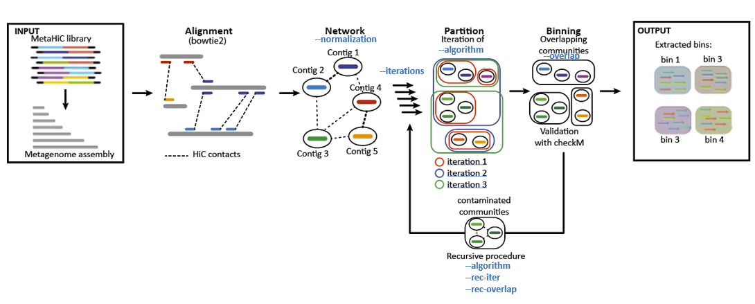
A lot of parameters could be modify to optimize the binning at your own datasets. The default parameters aare the one which usually give the best results. However, depending on your datasets and if you want to do a manual cleaning step to decontaminate your MAGs, some parameters could be optimize.
 metator_binning
a. Alignment
As previously explained, you cannot change directly the alignment parameters in MetaTOR yet. However, it’s possible to make your own alignment and start with your bam or pairs files. You can also preprocess your reads before if it’s necessary.
b. Network normalization
The normalization of metaHiC network is an important question. Currently, the default normalization consists in divided the number of inter-contig contacts by the geometric mean of the intra-contig contacts. It’s showing the best results according to our benchmark. However, if you want to do your own normalization using models such as the one proposed by HiCzin [5] which might yield better results you could do as follow:
# Build a network without normalization:
metator network -1 for.bam -2 rev.bam -a assembly.fa -n None
# Make your own network normalized (you just have to modify the third column of the network.txt file).
# Run the metaTOR pipleine at start stage network:
metator pipeline -n network_with_your_own_normalization.txt -a assembly.fa -S network
c. Partition parameters
For the partition you have 6 parameters that you can change. The default parameters have been choose as they usually work well on usual datasets. However, depending and your datasets you may want to change them:
The partition algorithm: either Louvain or Leiden algorithm. Louvain [Default: Louvain]
The resolution parameter of Leiden quality function (Constant Potts Model). The bigger the parameter is the more stringent the clusterization is (more bins will be created).
The number of iterations in the first partition. The more ierations you do the more bins you creates. Benchmark shows that 100 iterations are sufficient to extract all the bins. [Default: 100]
The number of iterations in the recursive partition. [Default: 10]
The overlapping parameter of the first partition. The overlapping parameters is the threshold percentage of iterations which bin two contigs in the same bin. A big overlapping parameter will reduce the contamination but bins might be uncomplete. [Default: 80]
The overlapping parameter of the recursive partition. [Default: 90]
D. Analysing the output
Some others tutorials are available to analyze the output:
References
[1] MetaTOR: A Computational Pipeline to Recover High-Quality Metagenomic Bins From Mammalian Gut Proximity-Ligation (meta3C) Libraries., L. Baudry, T. Foutel-Rodier, A. Thierry, R. Koszul, M. Marbouty. Frontiers in genetics, 2019.
[2] MEGAHIT: an ultra-fast single-node solution for large and complex metagenomics assembly via succinct de Bruijn graph, D. Li, C. Liu, R. Luo, Kunihiko Sadakane, T. Lam, Bioinformatics, 2015.
[3] Using SPAdes De Novo Assembler, A. Prjibelski, D. Antipov, D. Meleshko, A. Lapidus, A. Korobeynikov, Current Protocol in Bioinformatics, 2020.
[4] Hicstuff: Simple library/pipeline to generate and handle Hi-C data., C. Matthey-Doret, L. Baudry, A. Bignaud, A. Cournac, R. Montagne, N. Guiglielmoni, T. Foutel Rodier and V. F. Scolari, Zenodo, 2020.
[5] HiCzin: Normalizing metagenomic Hi-C data and detecting spurious contacts using zero-inflated negative binomial regression Y. Du, S. M. Laperriere, J. Fuhrman, F. Sun, bioRxiv, 2021.